July, 2013 | R-statistics blog

Analyzing Your Data on the AWS Cloud (with R)

Disclaimer:
This post is not intended to be a comprehensive review, but more of a “getting started guide”. If I did not mention an important tool or package I apologize, and invite readers to contribute in the comments.

Introduction

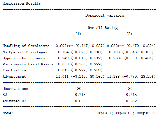
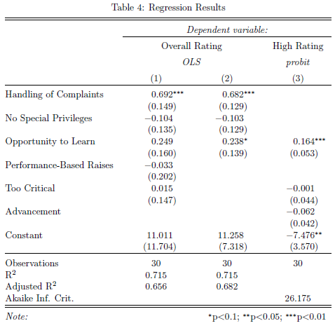
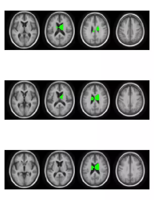
I have recently had the delight to participate in a “Brain Hackathon” organized as part of the OHBM2013 conference. Being supported by Amazon, the hackathon participants were provided with Amazon credit in order to promote the analysis using Amazon’s Web Services (AWS). We badly needed this computing power, as we had 14*10⁹ p-values to compute in order to localize genetic associations in the brain leading to Figure 1.

Figure 1- Brain volumes significantly associated to genotype.

While imaging genetics is an interesting research topic, and the hackathon was a great idea by itself, it is the AWS I wish to present in this post. Starting with the conclusion:

Storing your data and analyzing it on the cloud, be it AWS, Azure, Rackspace or others, is a quantum leap in analysis capabilities. I fell in love with my new cloud powers and I strongly recommend all statisticians and data scientists get friendly with these services. I will also note that if statisticians do not embrace these new-found powers, we should not be surprised if data analysis becomes synonymous with Machine Learning and not with Statistics (if you have no idea what I am talking about, read this excellent post by Larry Wasserman).

As motivation for analysis in the cloud consider:

The ability to do your analysis from any device, be it a PC, tablet or even smartphone.
The ability to instantaneously augment your CPU and memory to any imaginable configuration just by clicking a menu. Then scaling down to save costs once you are done.
The ability to instantaneously switch between operating systems and system configurations.
The ability to launch hundreds of machines creating your own cluster, parallelizing your massive job, and then shutting it down once done.

Here is a quick FAQ before going into the setup stages.

FAQ

Q: How does R fit in?

Continue reading “Analyzing Your Data on the AWS Cloud (with R)”

Tailor Your Tables with stargazer: New Features for LaTeX and Text Output

Guest post by Marek Hlavac

Since its first introduction on this blog, stargazer, a package for turning R statistical output into beautiful LaTeX and ASCII text tables, has made a great deal of progress. Compared to available alternatives (such as apsrtable or texreg), the latest version (4.0) of stargazer supports the broadest range of model objects. In particular, it can create side-by-side regression tables from statistical model objects created by packages AER, betareg, dynlm, eha, ergm, gee, gmm, lme4, MASS, mgcv, nlme, nnet, ordinal, plm, pscl, quantreg, relevent, rms, robustbase, spdep, stats, survey, survival and Zelig. You can install stargazer from CRAN in the usual way:

install.packages(“stargazer”)

New Features: Text Output and Confidence Intervals

In this blog post, I would like to draw attention to two new features of stargazer that make the package even more useful:

stargazer can now produce ASCII text output, in addition to LaTeX code. As a result, users can now create beautiful tables that can easily be inserted into Microsoft Word documents, published on websites, or sent via e-mail. Sharing your regression results has never been easier. Users can also use this feature to preview their LaTeX tables before they use the stargazer-generated code in their .tex documents.
In addition to standard errors, stargazer can now report confidence intervals at user-specified confidence levels (with a default of 95 percent). This possibility might be especially appealing to researchers in public health and biostatistics, as the reporting of confidence intervals is very common in these disciplines.

In the reproducible example presented below, I demonstrate these two new features in action.

Reproducible Example

I begin by creating model objects for two Ordinary Least Squares (OLS) models (using the lm() command) and a probit model (using glm() ). Note that I use data from attitude, one of the standard data frames that should be provided with your installation of R.

## 2 OLS models

linear.1 <- lm(rating ~ complaints + privileges + learning + raises + critical, data=attitude)
linear.2 <- lm(rating ~ complaints + privileges + learning, data=attitude)

## create an indicator dependent variable, and run a probit model

attitude$high.rating <- (attitude$rating > 70)
probit.model <- glm(high.rating ~ learning + critical + advance, data=attitude, family = binomial(link = "probit"))

I then use stargazer to create a ‘traditional’ LaTeX table with standard errors. With the sole exception of the argument no.space – which I use to save space by removing all empty lines in the table – both the command call and the resulting table should look familiar from earlier versions of the package:

stargazer(linear.1, linear.2, probit.model, title="Regression Results", align=TRUE, dep.var.labels=c("Overall Rating","High Rating"), covariate.labels=c("Handling of Complaints","No Special Privileges", "Opportunity to Learn","Performance-Based Raises","Too Critical","Advancement"), omit.stat=c("LL","ser","f"), no.space=TRUE)

Continue reading "Tailor Your Tables with stargazer: New Features for LaTeX and Text Output"

Creating good looking survival curves – the 'ggsurv' function

This is a guest post by Edwin Thoen

Currently I am doing my master thesis on multi-state models. Survival analysis was my favourite course in the masters program, partly because of the great survival package which is maintained by Terry Therneau. The only thing I am not so keen on are the default plots created by this package, by using plot.survfit. Although the plots are very easy to produce, they are not that attractive (as are most R default plots) and legends has to be added manually. I come across them all the time in the literature and wondered whether there was a better way to display survival. Since I was getting the grips of ggplot2 recently I decided to write my own function, with the same functionality as plot.survfitbut with a result that is much better looking. I stuck to the defaults of plot.survfit as much as possible, for instance by default plotting confidence intervals for single-stratum survival curves, but not for multi-stratum curves. Below you’ll find the code of the ggsurv function. Just as plot.survfit it only requires a fitted survival object to produce a default plot. We’ll use the lung data set from the survival package for illustration. First we load in the function to the console (see at the end of this post).

Once the function is loaded, we can get going, we use the lung data set from the survival package for illustration.

library(survival)
data(lung)
lung.surv <- survfit(Surv(time,status) ~ 1, data = lung)
ggsurv(lung.surv)

Continue reading "Creating good looking survival curves – the 'ggsurv' function"