The recent release of R 3.2.2 came with a small (but highly valuable) improvement to the stats:::labels.dendrogram function. When working with dendrograms with (say) 1000 labels, the new function offers a 70 times speed improvement over the version of the function from R 3.2.1. This speedup is even better than the Rcpp version of labels.dendrogram from the dendextendRcpp package.
Here is some R code to demonstrate this speed improvement:
# IF you are missing an of these - they should be installed:
install.packages("dendextend")
install.packages("dendextendRcpp")
install.packages("microbenchmark")


# Getting labels from dendextendRcpp
labelsRcpp% dist %>% hclust %>% as.dendrogram
labels(dend)
As we can see, the new labels function (in R 3.2.2) is about 70 times faster than the older version (from R 3.2.1). When only wanting something like the number of labels, using length on order.dendrogram will still be (about 3 times) faster than using labels.
R 3.2.2 (codename “Fire Safety”) was released last weekend. You can get the latest binaries version from here. (or the .tar.gz source code from here). The full list of new features and bug fixes is provided below.
SOME OF THE CHANGES
I personally found two things particularly interesting in this release:
Also, David Smith (from Revolution/Microsoft) highlighted in his post several of the updates in R 3.2.2 he found interesting – mentioning how the new default for accessing the web with R will rely on the HTTPS protocol, and of improving the accuracy in the extreme tails of the t and hypergeometric distributions.
Upgrading to R 3.2.2 on Windows
If you are using Windows you can easily upgrade to the latest version of R using the installr package. Simply run the following code in Rgui:
install.packages("installr") # install
setInternet2(TRUE)
installr::updateR() # updating R.
I try to keep the installr package updated and useful, so if you have any suggestions or remarks on the package – you are invited to open an issue in the github page.
CHANGES IN R 3.2.2:
SIGNIFICANT USER-VISIBLE CHANGES
It is now easier to use secure downloads from https:// URLs on builds which support them: no longer do non-default options need to be selected to do so. In particular, packages can be installed from repositories which offer https:// URLs, and those listed by setRepositories()now do so (for some of their mirrors).Support for https:// URLs is available on Windows, and on other platforms if support forlibcurl was compiled in and if that supports the https protocol (system installations can be expected to do). So https:// support can be expected except on rather old OSes (an example being OS X ‘Snow Leopard’, where a non-system version of libcurl can be used).(Windows only) The default method for accessing URLs viadownload.file() and url() has been changed to be "wininet" using Windows API calls. This changes the way proxies need to be set and security settings made: there have been some reports of sites being inaccessible under the new default method (but the previous methods remain available).
p.s.: Yes – this presentation is very similar, although not identical, to the one I gave at useR2015. For example, I mention the new bioinformatics paper on dendextend.
Summary:dendextend is an R package for creating and comparing visually appealing tree diagrams. dendextend provides utility functions for manipulating dendrogram objects (their color, shape, and content) as well as several advanced methods for comparing trees to one another (both statistically and visually). As such, dendextend offers a flexible framework for enhancing R’s rich ecosystem of packages for performing hierarchical clustering of items.
When using the dendextend package in your work, please cite it using:
Tal Galili (2015). dendextend: an R package for visualizing, adjusting, and comparing trees of hierarchical clustering. Bioinformatics. doi:10.1093/bioinformatics/btv428
My R package dendextend (version 1.0.1) is now on CRAN!
The dendextend package Offers a set of functions for extending dendrogram objects in R, letting you visualize and compare trees of hierarchical clusterings. With it you can (1) Adjust a tree’s graphical parameters – the color, size, type, etc of its branches, nodes and labels. (2) Visually and statistically compare different dendrograms to one another.
The previous release of dendextend (0.18.3) was half a year ago, and this version includes many new features and functions.
To help you discover how dendextend can solve your dendrogram/hierarchical-clustering issues, you may consult one of the following vignettes:
Here is an example figure from the first vignette (analyzing the Iris dataset)
This week, at useR!2015, I will give a talk on the package. This will offer a quick example, and a step-by-step example of some of the most basic/useful functions of the package. Here are the slides:
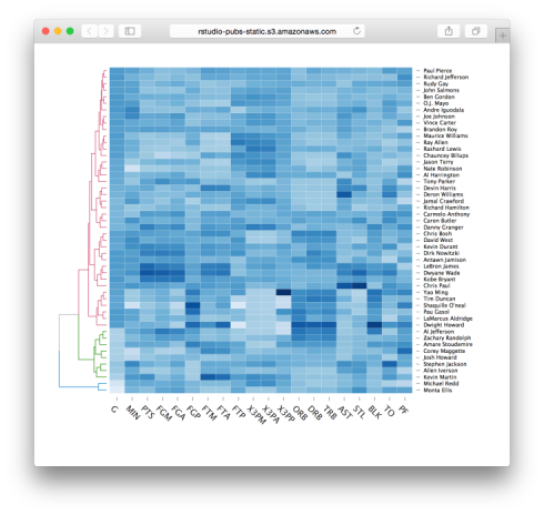
Lastly, I would like to mention the new d3heatmap package for interactive heat maps. This package is by Joe Cheng from Rstudio, and integrates well with dendrograms in general and dendextend in particular (thanks to some lovely github-commit-discussion between Joe and I). You are invited to see lively examples of the package in the post at the RStudio blog. Here is just one quick example:
Amazon Web Services (AWS) include many different computational tools, ranging from storage systems and virtual servers to databases and analytical tools. For us R-programmers, being familiar and experienced with these tools can be extremely beneficial in terms of efficiency, style, money-saving and more.
In this post we present a step-by-step screenshot tutorial that will get you to know Amazon EC2 service. We will set up an EC2 instance (Amazon virtual server), install an Rstudio server on it and use our beloved Rstudio via browser (all for free!). The slides below will also include an introduction to linux commands (basic), instructions for connecting to a remote server via ssh and more. No previous knowledge is required.
Useful links:
Set up an AWS account (do not worry about the credit card details, you will not be charged for any of our actions) – the steps are presented in the slides below.
Windows users: download MobaXterm (or any other ssh client software). Mac users: make sure you are familiar with the terminal (cause I’m not).
R 3.2.1 (codename “World-Famous Astronaut”) was released yesterday. You can get the latest binaries version from here. (or the .tar.gz source code from here). The full list of new features and bug fixes is provided below.
Upgrading to R 3.2.1 on Windows
If you are using Windows you can easily upgrade to the latest version of R using the installr package. Simply run the following code in Rgui:
install.packages("installr") # install
installr::updateR() # updating R.
I try to keep the installr package updated and useful, so if you have any suggestions or remarks on the package – you are invited to open an issue in the github page.
CHANGES IN R 3.2.1:
NEW FEATURES
utf8ToInt() now checks that its input is valid UTF-8 and returns NA if it is not.
install.packages() now allows type = "both" with repos = NULL if it can infer the type of file.
nchar(x, *) and nzchar(x) gain a new argument keepNA which governs how the result for NAs in x is determined. For the R 3.2.x series, the default remains FALSE which is fully back compatible. From R 3.3.0, the default will change to keepNA = NA and you are advised to consider this for code portability.
news() more flexibly extracts dates from package ‘NEWS.Rd’ files.
lengths(x) now also works (trivially) for atomic x and hence can be used more generally as an efficient replacement of sapply(x, length) and similar.
The included version of PCRE has been updated to 8.37, a bug-fix release.
diag() no longer duplicates a matrix when extracting its diagonal.
as.character.srcref() gains an argument to allow characters corresponding to a range of source references to be extracted.
If you are running R on Windows you can easily upgrade to the latest version of R using the installr package. Simply run the following code:
# installing/loading the latest installr package:
install.packages("installr"); library(installr) # install+load installr

updateR() # updating R.
Running “updateR()” will detect if there is a new R version available, and if so it will download+install it (etc.). just press “next”, “OK”, and “Yes” on everything…
A GUI interface to updating R on Windows
Starting from installr version 0.15.0, the upgradingprocess can be done with a click-on-menus GUI interface. Here is how to use it.
R 3.2.0 (codename “Full of Ingredients”) was released yesterday. You can get the latest binaries version from here. (or the .tar.gz source code from here). The full list of new features and bug fixes is provided below.
Upgrading to R 3.2.0 on Windows
If you are using Windows you can easily upgrade to the latest version of R using the installr package. Simply run the following code:
# installing/loading the latest installr package:
install.packages("installr"); library(installr) #load / install+load installr

updateR() # updating R.
Running “updateR()” will detect if there is a new R version available, and if so it will download+install it (etc.).
I try to keep the installr package updated and useful, so if you have any suggestions or remarks on the package – you are invited to leave a comment below.
CHANGES IN R 3.2.0:
As always, David smith mentioned in his post some of the main changes, writing how many of the changes in this release have happened behind the scenes to improve R’s engine for performance and reliability. These include:
A number of fixes proposed by Radford Neal, bringing some of the performance improvements of pqR to R while maintaining backwards compatibility.
more progress in handling big in-memory data objects (for example, you can now cbind/rbind matrices with more than 2 billion elements).
some significant updates to R’s byte compiler with new instructions that allow many scalar subsetting and assignment and scalar arithmetic operations to be handled more efficiently. This can result in significant performance improvements in scalar numerical code.
the package-checking system now does a more thorough job of making sure contributed packages comply with CRAN policies.
And here is also the full list of new features, bug fixes, etc:
(This is a guest post by my friend Yoni Sidi, a PhD candidate in statistics at the Hebrew University)
Background
The Israeli elections are coming up this Tuesday, 17/3/2015 (i.e.: tomorrow!). They are a bit more complicated than your average US presidential race. The elections in Israel are based on nationwide proportional representation. The electoral threshold is 3.25% and the number of seats (or mandates) out of a total of 120 is proportional to the number of votes it recieves, so the threshold roughly translates to at least four mandates. The Israeli system is a multi-party system and is based on coalition governments. Multi-party is putting it mildly, there are 11 that have a chance (and are expected) to pass the mandate threshold.
There are two major parties, Hamachane Hazioni (Left Wing) and the Likud (Right Wing), that are hoping to garner between 16%-25% of the votes, 20-30 mandates. The main winners though are the medium size parties that recomend to the President who they think has the best chance to construct the next government, so yes there is a good possibility that the general elections winner will not be one constructing the coalition. Making the actual winners the parties that create the biggest coalition which exceeds 60 mandates.
An abundance of polling has been continually published during the run up and the variaety of pollsters and publishers is hard to keep track of as a casual voter trying to gauge the temperature of the political landscape. I came across a great realtime database by Project 61 on google docs of past and present polling result information and decided that it was a great opportunity to learn the Shiny library of RStudio and create an app that I can check current and past results. So after I figured out how to connect google docs to R, I created a self updating app that became a nice place to keep track of polling every day, check trends and distributions using interactive ggplot2 graphs and simulate coalition outcomes.
Please note that as of Friday (March 13th), until election day (March 17th), it is forbidden to perform new polls in Israel, hence the data presented here cannot allow for an up-to-date inference about the expected results of the election. This post is for educational purposes.
Running the election polls Shiny app on your computer
#changing locale to run on Windows
if (Sys.info()[1] == "Windows") Sys.setlocale("LC_ALL","Hebrew_Israel.1255")

#check to see if libraries need to be installed
libs <- c("shiny","shinyAce","httr","XML","stringr","ggplot2","scales","plyr","reshape2","dplyr")
x <- sapply(libs,function(x)if(!require(x,character.only = T)) install.packages(x))
rm(x,libs)

#run App
shiny::runGitHub("Elections","yonicd",subdir="shiny")

#reset to original locale on Windows
if (Sys.info()[1] == "Windows") Sys.setlocale("LC_ALL")
The latest polling day results published in the media and the prediction made using the Project 61 weighting schemes. The parties are stacked into blocks to see which block has best chance to create a coalition.
The Project 61 prediction is based past pollster error deriving weights from the 2003,2006,2009 and 2013 elections, dependant on days to elections and parties. In their site there is an extensive analysis on pollster bias towards certain parties and party blocks.
Election Analysis
An interactive polling analysis layout where the user can filter elections, parties, publishers and pollster, dates and create different types of plots using any variable as the x and y axis.
The default layer is the 60 day trend (estimated with loess smoother) of mandates published by each pollster by party
The user can choose to include in the plots Elections (2003,2006,2009,2013,2015) and the subsequent filters are populated with the relevant parties, pollsters and publishers relevant to the chosen elections. Next there is a slider to choose the days before the election you want to view in the plot. This was used instead of a calendar to make a uniform timeline when comparing across elections.
In addition the plot itself is a ggplot thus the options above the graph give the user control on nearly all the options to build a plot. The user can choose from the following variables:
Time
Party
Results
Poll
Election
Party
Mandates
Publisher
DaysLeft
Ideology (5 Party Blocks)
Mandate.Group
Pollster
Date
Ideology.Group (2 Party Blocks)
Results
year
Attribute (Party History)
(Pollster) Error
month
week
To define the following plot attributes:
Plot Type
Axes
Grouping
Plot Facets
Point
X axis variable
Split Y by colors using a different variable
Row Facet
Bar
Discrete/Continuous
Column Facet
Line
Rotation of X tick labels
Step
Y axis variable
Boxplot
Density
Create Facets to display subsets of the data in different panels (two more variables to cut data) there are two type of facets to choose from
Wrap: Wrap 1d ribbon of panels into 2d
Grid: Layout panels in a grid (matrix)
An example of filtering pollsters to compare different tendencies for each party in the 2015 elections:
An example of comparing distribution mandates per party in the last two months of polling
An example of comparing distribution of pollster errors across elections (up to 10 days prior end of polling), by splitting the parties into five groups compared to previous election: old party,new party, combined (combination of two or more old parties), new.split (new party created from a split of a party from last election), old.split (old party that was a left from the split).
As we can see the pollster do not get a good indication of new,new.split or combined parties, which could be a problem this election since there are: 3 combined, 2 new splits.
If you are an R user and know ggplot there is an additional editor console,below the plot, where you can create advanced plots freehand, just add to the final object from the GUI called p and the data.frame is x, eg p+geom_point(). Just notice that all aesthetics must be given they are not defined in the original ggplot() definition. It is also possible to use any library you want just add it to the top of the code, the end object must be a ggplot.
You can also remove the original layer if you want using the function remove_geom(ggplot_object,geom_layer), eg p=p+remove_geom(p,“point”) will remove the geom_point layer in the original graph
p=remove_geom(p,"point")#blank ggplot with facets in place#new layerp+geom_smooth(aes(x=DaysLeft,y=Mandates,fill=Party.En))+scale_x_reverse()+scale_fill_discrete(name="Party")
Finally the plots can be viewed in English or Hebrew, and can be downloaded to you local computer using the download button.
Mandate Simulator and Coalition Whiteboard
A bootstrap simulation is run on Polling results from up to 10 of the latest polls using the sampling error as the uncertainty of each mandate published. Taking into account mandate surplus agreements using the Hagenbach-Bischoff quota method and the mandate threshold limit (in this election it is 4 mandates), calculating the simulated final tally of mandates. The distributions are plotted per party and the location of the median published results in the media.
The user can choose how many polls to take into account, up to last 10 polls, and how big a simulation they want to run: 50,100,500,1000 random polling results per each party and poll.
Once the simulator is complete you can create coalitions based on either the simulated distribution or actual published polls and see who can pass 60 mandates. Choose the coalition parties and the opposition parties from dropdown lists. (Yes the ones chosen are nonsensical on purpose…)
Polling Database
All raw data used in the application can be viewed and filtered in a datatable.