R 3.2.4 is released

R 3.2.4 (codename “Very Secure Dishes”) was released today. You can get the latest binaries version from here. (or the .tar.gz source code from here). The full list of new features and bug fixes is provided below.

Upgrading to R 3.2.4 on Windows

If you are using Windows you can easily upgrade to the latest version of R using the installr package. Simply run the following code in Rgui:

install.packages("installr") # install 
setInternet2(TRUE)
installr::updateR() # updating R.

Running “updateR()” will detect if there is a new R version available, and if so it will download+install it (etc.). There is also a step by step tutorial (with screenshots) on how to upgrade R on Windows, using the installr package.

I try to keep the installr package updated and useful, so if you have any suggestions or remarks on the package – you are invited to open an issue in the github page.

NEW FEATURES

  • install.packages() and related functions now give a more informative warning when an attempt is made to install a base package.
  • summary(x) now prints with less rounding when x contains infinite values. (Request of PR#16620.)
  • provideDimnames() gets an optional unique argument.
  • shQuote() gains type = "cmd2" for quoting in cmd.exe in Windows. (Response to PR#16636.)
  • The data.frame method of rbind() gains an optional argument stringsAsFactors (instead of only depending on getOption("stringsAsFactors")).
  • smooth(x, *) now also works for long vectors.
  • tools::texi2dvi() has a workaround for problems with the texi2dvi script supplied by texinfo 6.1.

    It extracts more error messages from the LaTeX logs when in emulation mode.

UTILITIES

  • R CMD check will leave a log file ‘build_vignettes.log’ from the re-building of vignettes in the ‘.Rcheck’ directory if there is a problem, and always if environment variable_R_CHECK_ALWAYS_LOG_VIGNETTE_OUTPUT_ is set to a true value.

DEPRECATED AND DEFUNCT

  • Use of SUPPORT_OPENMP from header ‘Rconfig.h’ is deprecated in favour of the standard OpenMP define _OPENMP.

    (This has been the recommendation in the manual for a while now.)

  • The make macro AWK which is long unused by R itself but recorded in file ‘etc/Makeconf’ is deprecated and will be removed in R 3.3.0.
  • The C header file ‘S.h’ is no longer documented: its use should be replaced by ‘R.h’.

BUG FIXES

  • kmeans(x, centers = <1-row>) now works. (PR#16623)
  • Vectorize() now checks for clashes in argument names. (PR#16577)
  • file.copy(overwrite = FALSE) would signal a successful copy when none had taken place. (PR#16576)
  • ngettext() now uses the same default domain as gettext(). (PR#14605)
  • array(.., dimnames = *) now warns about non-list dimnames and, from R 3.3.0, will signal the same error for invalid dimnames as matrix() has always done.
  • addmargins() now adds dimnames for the extended margins in all cases, as always documented.
  • heatmap() evaluated its add.expr argument in the wrong environment. (PR#16583)
  • require() etc now give the correct entry of lib.loc in the warning about an old version of a package masking a newer required one.
  • The internal deparser did not add parentheses when necessary, e.g. before [] or [[]]. (Reported by Lukas Stadler; additional fixes included as well).
  • as.data.frame.vector(*, row.names=*) no longer produces ‘corrupted’ data frames from row names of incorrect length, but rather warns about them. This will become an error.
  • url connections with method = "libcurl" are destroyed properly. (PR#16681)
  • withCallingHandler() now (again) handles warnings even during S4 generic’s argument evaluation. (PR#16111)
  • deparse(..., control = "quoteExpressions") incorrectly quoted empty expressions. (PR#16686)
  • format()ting datetime objects ("POSIX[cl]?t") could segfault or recycle wrongly. (PR#16685)
  • plot.ts(<matrix>, las = 1) now does use las.
  • saveRDS(*, compress = "gzip") now works as documented. (PR#16653)
  • (Windows only) The Rgui front end did not always initialize the console properly, and could cause R to crash. (PR#16998)
  • dummy.coef.lm() now works in more cases, thanks to a proposal by Werner Stahel (PR#16665). In addition, it now works for multivariate linear models ("mlm", manova) thanks to a proposal by Daniel Wollschlaeger.
  • The as.hclust() method for "dendrogram"s failed often when there were ties in the heights.
  • reorder() and midcache.dendrogram() now are non-recursive and hence applicable to somewhat deeply nested dendrograms, thanks to a proposal by Suharto Anggono in PR#16424.
  • cor.test() now calculates very small p values more accurately (affecting the result only in extreme not statistically relevant cases). (PR#16704)
  • smooth(*, do.ends=TRUE) did not always work correctly in R versions between 3.0.0 and 3.2.3.
  • pretty(D) for date-time objects D now also works well if range(D) is (much) smaller than a second. In the case of only one unique value in D, the pretty range now is more symmetric around that value than previously.
    Similarly, pretty(dt) no longer returns a length 5 vector with duplicated entries for Date objects dt which span only a few days.
  • The figures in help pages such as ?points were accidentally damaged, and did not appear in R 3.2.3. (PR#16708)
  • available.packages() sometimes deleted the wrong file when cleaning up temporary files. (PR#16712)
  • The X11() device sometimes froze on Red Hat Enterprise Linux 6. It now waits for MapNotify events instead of Expose events, thanks to Siteshwar Vashisht. (PR#16497)
  • [dpqr]nbinom(*, size=Inf, mu=.) now works as limit case, for ‘dpq’ as the Poisson. (PR#16727)
    pnbinom() no longer loops infinitely in border cases.
  • approxfun(*, method="constant") and hence ecdf() which calls the former now correctly “predict” NaN values as NaN.
  • summary.data.frame() now displays NAs in Date columns in all cases. (PR#16709)


logo

It’s not the p-values’ fault – reflections on the recent ASA statement (+relevant R resources)

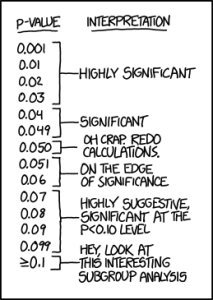
Joint post by Yoav Benjamini and Tal Galili. The post highlights points raised by Yoav in his official response to the ASA statement (available as on page 4 in the ASA supplemental tab), as well as offers a list of relevant R resources.

Summary

The ASA statement about the misuses of the p-value singles it out. It is just as well relevant to the use of most other statistical methods: context matters, no single statistical measure suffices, specific thresholds should be avoided and reporting should not be done selectively. The latter problem is discussed mainly in relation to omitted inferences. We argue that the selective reporting of inferences problem is serious enough a problem in our current industrialized science even when no omission takes place. Many R tools are available to address it, but they are mainly used in very large problems and are grossly underused in areas where lack of replicability hits hard.

p_valuesSource: xkcd

Continue reading “It’s not the p-values’ fault – reflections on the recent ASA statement (+relevant R resources)”

50 years of Data Science – by David Donoho

David Donoho published a fascinating paper based on a presentation at the Tukey Centennial workshop, Princeton NJ Sept 18 2015. You can download the full paper from here. 

The paper got quite the attention on Hacker News, Data Science Central, Simply Stats, Xi’an’s blog, srown ion medium, and probably others. Share your thoughts in the comments.

Here is the abstract and table of content.

Abstract

More than 50 years ago, John Tukey called for a reformation of academic statistics. In ‘The Future of Data Analysis’, he pointed to the existence of an as-yet unrecognized science, whose subject of interest was learning from data, or ‘data analysis’. Ten to twenty years ago, John Chambers, Bill Cleveland and Leo Breiman independently once again urged academic statistics to expand its boundaries beyond the classical domain of theoretical statistics; Chambers called for more emphasis on data preparation and presentation rather than statistical modeling; and Breiman called for emphasis on prediction rather than inference. Cleveland even suggested the catchy name “Data Science” for his envisioned field.

A recent and growing phenomenon is the emergence of “Data Science” programs at major universities, including UC Berkeley, NYU, MIT, and most recently the Univ. of Michigan, which on September 8, 2015 announced a $100M “Data Science Initiative” that will hire 35 new faculty. Teaching in these new programs has significant overlap in curricular subject matter with traditional statistics courses; in general, though, the new initiatives steer away from close involvement with academic statistics departments.

This paper reviews some ingredients of the current “Data Science moment”, including recent commentary about data science in the popular media, and about how/whether Data Science is really different from Statistics.

The now-contemplated field of Data Science amounts to a superset of the fields of statistics and machine learning which adds some technology for ‘scaling up’ to ‘big data’. This chosen superset is motivated by commercial rather than intellectual developments. Choosing in this way is likely to miss out on the really important intellectual event of the next fifty years.

Because all of science itself will soon become data that can be mined, the imminent revolution in Data Science is not about mere ‘scaling up’, but instead the emergence of scientific studies of data analysis science-wide. In the future, we will be able to predict how a proposal to change data analysis workflows would impact the validity of data analysis across all of science, even predicting the impacts field-by-field. Drawing on work by Tukey, Cleveland, Chambers and Breiman, I present a vision of data science based on the activities of people who are ‘learning from data’, and I describe an academic field dedicated to improving that activity in an evidence-based manner. This new field is a better academic enlargement of statistics and machine learning than today’s Data Science Initiatives, while being able to accommodate the same short-term goals.

Contents

1 Today’s Data Science Moment

2 Data Science ‘versus’ Statistics

2.1 The ‘Big Data’ Meme

2.2 The ‘Skills’ Meme

2.3 The ‘Jobs’ Meme

2.4 What here is real?

2.5 A Better Framework

3 The Future of Data Analysis, 1962

4 The 50 years since FoDA

4.1 Exhortations

4.2 Reification

5 Breiman’s ‘Two Cultures’, 2001

6 The Predictive Culture’s Secret Sauce

6.1 The Common Task Framework

6.2 Experience with CTF

6.3 The Secret Sauce

6.4 Required Skills

7 Teaching of today’s consensus Data Science

8 The Full Scope of Data Science

8.1 The Six Divisions

8.2 Discussion

8.3 Teaching of GDS

8.4 Research in GDS

8.4.1 Quantitative Programming Environments: R

8.4.2 Data Wrangling: Tidy Data

8.4.3 Research Presentation: Knitr

8.5 Discussion

9 Science about Data Science

9.1 Science-Wide Meta Analysis

9.2 Cross-Study Analysis

9.3 Cross-Workflow Analysis

9.4 Summary

10 The Next 50 Years of Data Science

10.1 Open Science takes over

10.2 Science as data

10.3 Scientific Data Analysis, tested Empirically

10.3.1 DJ Hand (2006)

10.3.2 Donoho and Jin (2008)

10.3.3 Zhao, Parmigiani, Huttenhower and Waldron (2014)

10.4 Data Science in 2065

11 Conclusion

You can download the full paper from here. 

Multidimensional Scaling with R (from “Mastering Data Analysis with R”)

Guest post by Gergely Daróczi. If you like this content, you can buy the full 396 paged e-book for 5 USD until January 8, 2016 as part of Packt’s “$5 Skill Up Campaign” at https://bit.ly/mastering-R

Feature extraction tends to be one of the most important steps in machine learning and data science projects, so I decided to republish a related short section from my intermediate book on how to analyze data with R. The 9th chapter is dedicated to traditional dimension reduction methods, such as Principal Component Analysis, Factor Analysis and Multidimensional Scaling — from which the below introductory examples will focus on that latter.

Multidimensional Scaling (MDS) is a multivariate statistical technique first used in geography. The main goal of MDS it is to plot multivariate data points in two dimensions, thus revealing the structure of the dataset by visualizing the relative distance of the observations. Multidimensional scaling is used in diverse fields such as attitude study in psychology, sociology or market research.

Although the MASS package provides non-metric methods via the isoMDS function, we will now concentrate on the classical, metric MDS, which is available by calling the cmdscale function bundled with the stats package. Both types of MDS take a distance matrix as the main argument, which can be created from any numeric tabular data by the dist function.

But before such more complex examples, let’s see what MDS can offer for us while working with an already existing distance matrix, like the built-in eurodist dataset:

> as.matrix(eurodist)[1:5, 1:5]
          Athens Barcelona Brussels Calais Cherbourg
Athens         0      3313     2963   3175      3339
Barcelona   3313         0     1318   1326      1294
Brussels    2963      1318        0    204       583
Calais      3175      1326      204      0       460
Cherbourg   3339      1294      583    460         0

The above subset (first 5-5 values) of the distance matrix represents the travel distance between 21 European cities in kilometers. Running classical MDS on this example returns:

> (mds <- cmdscale(eurodist))
                      [,1]      [,2]
Athens           2290.2747  1798.803
Barcelona        -825.3828   546.811
Brussels           59.1833  -367.081
Calais            -82.8460  -429.915
Cherbourg        -352.4994  -290.908
Cologne           293.6896  -405.312
Copenhagen        681.9315 -1108.645
Geneva             -9.4234   240.406
Gibraltar       -2048.4491   642.459
Hamburg           561.1090  -773.369
Hook of Holland   164.9218  -549.367
Lisbon          -1935.0408    49.125
Lyons            -226.4232   187.088
Madrid          -1423.3537   305.875
Marseilles       -299.4987   388.807
Milan             260.8780   416.674
Munich            587.6757    81.182
Paris            -156.8363  -211.139
Rome              709.4133  1109.367
Stockholm         839.4459 -1836.791
Vienna            911.2305   205.930

These scores are very similar to two principal components (discussed in the previous, Principal Component Analysis section), such as running prcomp(eurodist)$x[, 1:2]. As a matter of fact, PCA can be considered as the most basic MDS solution.

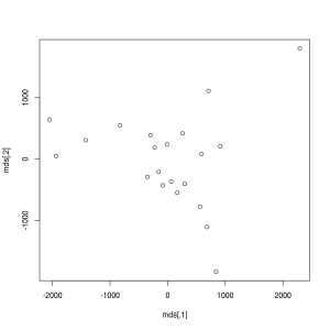
Anyway, we have just transformed (reduced) the 21-dimensional space into 2 dimensions, which can be plotted very easily — unlike the original distance matrix with 21 rows and 21 columns:

> plot(mds)

2028OS_09_16

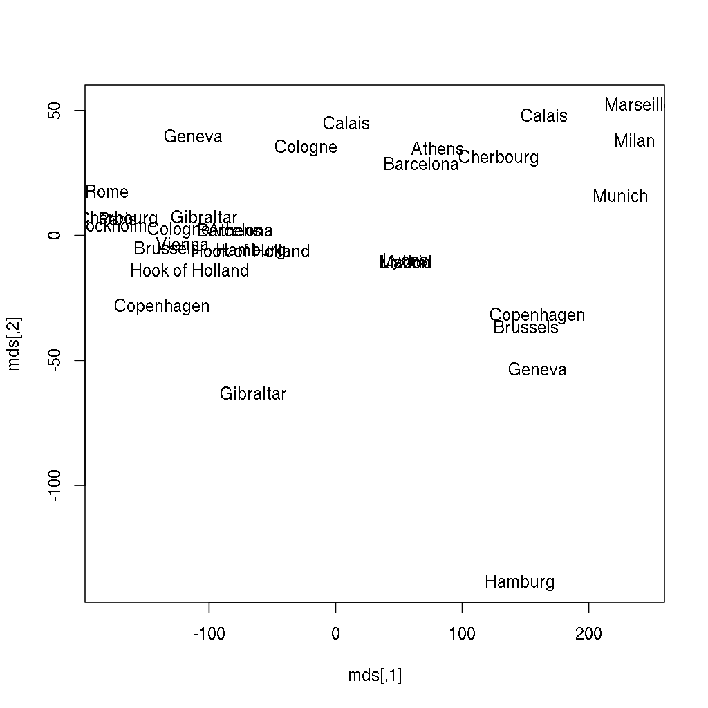
Does it ring a bell? If not yet, the below image might be more helpful, where the following two lines of code also renders the city names instead of showing anonymous points:

> plot(mds, type = 'n')
> text(mds[, 1], mds[, 2], labels(eurodist))
2028OS_09_17

Continue reading “Multidimensional Scaling with R (from “Mastering Data Analysis with R”)”