This is (roughly) the lightning talk I gave in useR2011. If you are a reader of R-bloggers.com then this talk is not likely to tell you anything new. However, if you have a friend, college or student who is a new useRs of R, this talk will offer him a decent introduction to what the R […]
This is (roughly) the lightning talk I gave in useR2011. If you are a reader of R-bloggers.com then this talk is not likely to tell you anything new. However, if you have a friend, college or student who is a new useRs of R, this talk will offer him a decent introduction to what the R blogosphere is all about.
The talk is a call for people of the R community to participate more in reading, writing and interacting with blogs.
I was encouraged to record this talk per the request of Chel Hee Lee, so it may be used in the recent useR conference in Korea (2011)
The talk (briefly) goes through:
The widespread influence of the R blogosphere
What R bloggers write about
How to encourage a blogger you enjoy reading to keep writing
How to start your own R blog (just go to wordpress.com)
And two thoughts about the future of R blogging (more bloggers and readers, and more interactive online visualization)
My apologies for any of the glitches in my English. For more talks about R, you can visit the R user groups blog. I hope more speakers from useR 2011 will consider uploading their talks online.
A guest post by Paul Hiemstra. ———— Fortran and C programmers often say that interpreted languages like R are nice and all, but lack in terms of speed. How fast something works in R greatly depends on how it is implemented, i.e. which packages/functions does one use. A prime example, which shows up regularly on […]
Fortran and C programmers often say that interpreted languages like R are nice and all, but lack in terms of speed. How fast something works in R greatly depends on how it is implemented, i.e. which packages/functions does one use. A prime example, which shows up regularly on the R-help list, is letting a vector grow as you perform an analysis. In pseudo-code this might look like:
1
2
3
4
5
dum = NULL
for(i in1:100000){# new_outcome = ...do some stuff...
dum =c(dum, new_outcome)}
The problem here is that dum is continuously growing in size. This forces the operating system to allocate new memory space for the object, which is terribly slow. Preallocating dum to the length it is supposed to be greatly improves the performance. Alternatively, the use of apply type of functions, or functions from plyr package prevent these kinds of problems. But even between more advanced methods there are large differences between different implementations.
Take the next example. We create a dataset which has two columns, one column with values (e.g. amount of rainfall) and in the other a category (e.g. monitoring station id). We would like to know what the mean value is per category. One way is to use for loops, but I’ll skip that one for now. Three possibilities exist that I know of: ddply (plyr), ave (base R) and data.table. The piece of code at the end of this post compares these three methods. The outcome in terms of speed is: (press the image to see a larger version)
It is quite obvious that ddply performs very bad when the number of unique categories is large. The ave function performs better. However, the data.table option is by far the best one, outperforming both other alternatives easily. In response to this, Hadley Wickham (author of plyr) responded:
This is a drawback of the way that ddply always works with data frames. It will be a bit faster if you use summarise instead of data.frame (because data.frame is very slow), but I’m still thinking about how to overcome this fundamental limitation of the ddply approach.
I hope this comparison is of use to readers. And remember, think before complaining that R is slow .
The news of the new release of R 2.13.0 is out, and the R blogosphere is buzzing. Bloggers posting excitedly about the new R compiler package that brings with it the hope to speed up our R code with up to 4 times improvement and even a JIT compiler for R. So it is time to upgrade, and bloggers are here to help. Some wrote how to upgrade R on Linux and mac OSX (based on posts by Paolo). And it is now my turn, with suggestions on how to upgrade R on windows 7.
There are basically two strategies for R upgrading on windows. The first is to install a new R version and copy paste all the packages to the new R installation folder. The second is to have a global R package folder, each time synced to the most current R installation (thus saving us the time of copying the package library each we upgrade R).
p.s: If this is the first time you are upgrading R using this method, then first run the following two lines on your old R installation (before running the above code in the new R intallation):
The above code should be enough. However, there are some common pitfalls you might encounter when upgrading R on windows 7, bellow I outline the ones I know about, and how they can be solved.
So it is no surprise that the new release of plyr 1.5 got me curious. While going through the news file with the new features and bug fixes, I noticed how (quietly) Hadley has also released (6 days ago) another version of plyr prior to 1.5 which was numbered 1.4.1. That version included only one more function, but a very important one – a new citation reference for when using the plyr package. Here is how to use it:
install.packages("plyr") # so to upgrade to the latest release
citation("plyr")
The output gives both a simple text version as well as a BibTeX entry for LaTeX users. Here it is (notice the download link for yourself to read):
To cite plyr in publications use: Hadley Wickham (2011). The Split-Apply-Combine Strategy for Data Analysis. Journal of Statistical Software, 40(1), 1-29. URL http://www.jstatsoft.org/v40/i01/.
I hope to see more R contributers and users will make use of the ?citation() function in the future.
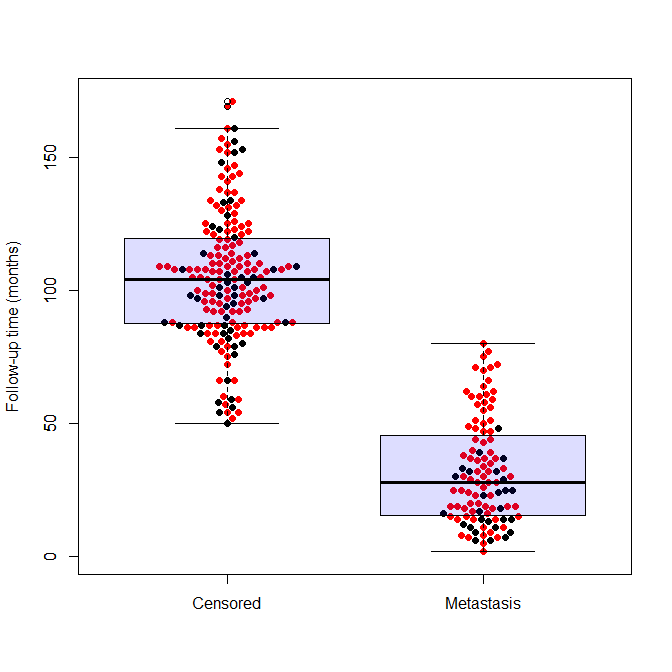
2016-05-28 update: I strongly recommend reading the comment by Leland Wilkinson. In summary, “beeswarm” plots are not recommended as they often create visual artifacts that distracts from the estimated density of the observations.
(The image above is called a “Beeswarm Boxplot” , the code for producing this image is provided at the end of this post)
The above plot is implemented under different names in different softwares. This “Scatter Dot Beeswarm Box Violin – plot” (in the lack of an agreed upon term) is a one-dimensional scatter plot which is like “stripchart”, but with closely-packed, non-overlapping points; the positions of the points are corresponding to the frequency in a similar way as the violin-plot. The plot can be superimposed with a boxplot to give a very rich description of the underlaying distribution.
This plot has been implemented in various statistical packages, in this post I will list the few I came by so far. And if you know of an implementation I’ve missed please tell me about it in the comments.
Recently I was asked by O’Reilly publishing to give a book review for Paul Teetor new introductory book to R. After giving the book some attention and appreciating it’s delivery of the material, I was happy to write and post this review. Also, I’m very happy to see how a major publishing house like O’Reilly is producing more and more R books, great news indeed.
And now for the book review:
Executive summary: a book that offers a well designed gentle introduction for people with some background in statistics wishing to learn how to get common (basic) tasks done with R.
Information
By: Paul Teetor Publisher:O’Reilly MediaReleased: January 2011 Pages: 58 (est.)
Format
The book “25 Recipes for Getting Started with R” offers an interesting take on how to bring R to the general (statistically oriented) public.
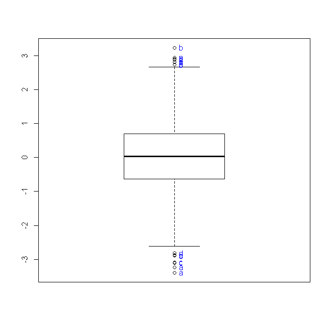
In this post I offer an alternative function for boxplot, which will enable you to label outlier observations while handling complex uses of boxplot.
In this post I present a function that helps to label outlier observations When plotting a boxplot using R.
An outlier is an observation that is numerically distant from the rest of the data. When reviewing a boxplot, an outlier is defined as a data point that is located outside the fences (“whiskers”) of the boxplot (e.g: outside 1.5 times the interquartile range above the upper quartile and bellow the lower quartile).
Identifying these points in R is very simply when dealing with only one boxplot and a few outliers. That can easily be done using the “identify” function in R. For example, running the code bellow will plot a boxplot of a hundred observation sampled from a normal distribution, and will then enable you to pick the outlier point and have it’s label (in this case, that number id) plotted beside the point:
set.seed(482)
y <- rnorm(100)
boxplot(y)
identify(rep(1, length(y)), y, labels = seq_along(y))
However, this solution is not scalable when dealing with:
Many outliers
Overlapping data-points, and
Multiple boxplots in the same graphic window
For such cases I recently wrote the function "boxplot.with.outlier.label" (which you can download from here). This function will plot operates in a similar way as "boxplot" (formula) does, with the added option of defining "label_name". When outliers are presented, the function will then progress to mark all the outliers using the label_name variable. This function can handle interaction terms and will also try to space the labels so that they won't overlap (my thanks goes to Greg Snow for his function "spread.labs" from the {TeachingDemos} package, and helpful comments in the R-help mailing list).
Here is some example code you can try out for yourself:
source("https://raw.githubusercontent.com/talgalili/R-code-snippets/master/boxplot.with.outlier.label.r") # Load the function
# sample some points and labels for us:
set.seed(492)
y <- rnorm(2000)
x1 <- sample(letters[1:2], 2000,T)
x2 <- sample(letters[1:2], 2000,T)
lab_y <- sample(letters[1:4], 2000,T)
# plot a boxplot with interactions:
boxplot.with.outlier.label(y~x2*x1, lab_y)
Here is the resulting graph:
You can also have a try and run the following code to see how it handles simpler cases:
# plot a boxplot without interactions:
boxplot.with.outlier.label(y~x1, lab_y, ylim = c(-5,5))
# plot a boxplot of y only
boxplot.with.outlier.label(y, lab_y, ylim = c(-5,5))
boxplot.with.outlier.label(y, lab_y, spread_text = F) # here the labels will overlap (because I turned spread_text off)
Here is the output of the last example, showing how the plot looks when we allow for the text to overlap (we would often prefer to NOT allow it).
Regarding package dependencies: notice that this function requires you to first install the packages {TeachingDemos} (by Greg Snow) and {plyr} (by Hadley Wickham)
Updates: 19.04.2011 - I've added support to the boxplot "names" and "at" parameters.
You are very much invited to leave your comments if you find a bug, think of ways to improve the function, or simply enjoyed it and would like to share it with me.
Rob Calver wrote an interesting invitation on the R mailing list today, inviting potential authors to submit their vision of the next great book about R. The announcement originated from the Chapman & Hall/CRC publishing houses, backed up by an impressive team of R celebrities, chosen as the editors of this new R books series, including:
A year ago (on December 9th 2009), I wrote about founding R-bloggers.com, an (unofficial) online R journal written by bloggers who agreed to contribute their R articles to the site.
In this post I wish to celebrate R-bloggers’ first birthday by sharing with you:
Links to the top 14 posts of 2010
Reflections about the origin of R-bloggers
Statistics on “how well” R-bloggers did this year
Links to other related projects
An invitation for sponsors/supporters to help keep the site alive


")