heatmaply: an R package for creating interactive cluster heatmaps for online publishing

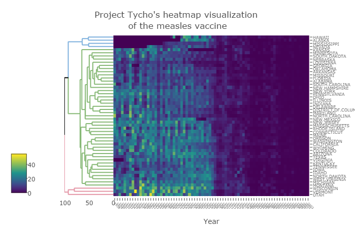
This post on the heatmaply package is based on my recent paper from the journal bioinformatics (a link to a stable DOI). The paper was published just last week, and since it is released as CC-BY, I am permitted (and delighted) to republish it here in full. My co-authors for this paper are Jonathan Sidi, Alan O’Callaghan, and Carson Sievert.

Summary: heatmaply is an R package for easily creating interactive cluster heatmaps that can be shared online as a stand-alone HTML file. Interactivity includes a tooltip display of values when hovering over cells, as well as the ability to zoom in to specific sections of the figure from the data matrix, the side dendrograms, or annotated labels.  Thanks to the synergistic relationship between heatmaply and other R packages, the user is empowered by a refined control over the statistical and visual aspects of the heatmap layout.

Availability: The heatmaply package is available under the GPL-2 Open Source license. It comes with a detailed vignette, and is freely available from: http://cran.r-project.org/package=heatmaply

Continue reading “heatmaply: an R package for creating interactive cluster heatmaps for online publishing”

Data Driven Cheatsheets

Guest post by Jonathan Sidi

Cheatsheets are currently built and used exclusivley as a teaching tool. We want to try and change this and produce a cheat sheet that gives a roadmap to build a known product, but also is built as a function so users can input data into it to make the cheatsheet more personalized. This gives a versalility of a consistent format that people can share with each other, but has the added value of conveying a message through data driven visual changes.

Example

ggplot2 themes

The ggplot2 theme object is an amazing object you can specify nearly any part of the plot that is not conditonal on the data. What sets the theme object apart is that its structure is consistent, but the values in it change. In addition to change a theme it is a single function that too has a consistent call. The reoccuring challenge for users is to remember all the options that can be used in the theme call (there are approximately 220 unique options to calibrate at last count) or bookmark the help page for the theme and remember how you deciphered it last time.

This becomes a problem to pass all the information of the theme to someone who does not know what the values are set in your theme and attach instructions on it to let them recreate it without needing to open any web pages.

In writing the library ggedit we tried to make it easy to edit your theme so you don’t have to know too much about ggplots to make a large number of changes at once, for a quick clip see here. We had to make it easy to track those changes for people who are not versed in R, and plot.theme() was the outcome. In short think of the theme as a lot of small images that are combined to create a singel portrait.

Continue reading “Data Driven Cheatsheets”

ggedit – interactive ggplot aesthetic and theme editor

Guest post by Jonathan Sidi, Metrum Research Group

ggplot2 has become the standard of plotting in R for many users. New users, however, may find the learning curve steep at first, and more experienced users may find it challenging to keep track of all the options (especially in the theme!).

ggedit is a package that helps users bridge the gap between making a plot and getting all of those pesky plot aesthetics just right, all while keeping everything portable for further research and collaboration.

ggedit is powered by a Shiny gadget where the user inputs a ggplot plot object or a list of ggplot objects. You can run ggedit directly from the console from the Addin menu within RStudio.

Continue reading “ggedit – interactive ggplot aesthetic and theme editor”

R 3.3.0 is released!

R 3.3.0 (codename “Supposedly Educational”) was released today. You can get the latest binaries version from here. (or the .tar.gz source code from here). The full list of new features and bug fixes is provided below.

Upgrading to R 3.3.0 on Windows

If you are using Windows you can easily upgrade to the latest version of R using the installr package. Simply run the following code in Rgui:

install.packages("installr") # install 
setInternet2(TRUE)
installr::updateR() # updating R.

Running “updateR()” will detect if there is a new R version available, and if so it will download+install it (etc.). There is also a step by step tutorial (with screenshots) on how to upgrade R on Windows, using the installr package. If you only see the option to upgrade to an older version of R, then change your mirror or try again in a few hours (it usually take around 24 hours for all CRAN mirrors to get the latest version of R).

I try to keep the installr package updated and useful, so if you have any suggestions or remarks on the package – you are invited to open an issue in the github page.

CHANGES IN R 3.3.0

SIGNIFICANT USER-VISIBLE CHANGES

  • nchar(x, *)‘s argument keepNA governing how the result for NAs in x is determined, gets a new default keepNA = NA which returns NA where x is NA, except for type = "width" which still returns 2, the formatting / printing width of NA.
  • All builds have support for https: URLs in the default methods for download.file(), url() and code making use of them.Unfortunately that cannot guarantee that any particular https: URL can be accessed. For example, server and client have to successfully negotiate a cryptographic protocol (TLS/SSL, …) and the server’s identity has to be verifiable via the available certificates. Different access methods may allow different protocols or use private certificate bundles: we encountered a https: CRAN mirror which could be accessed by one browser but not by another nor by download.file() on the same Linux machine.

NEW FEATURES

Continue reading “R 3.3.0 is released!”

labels.dendrogram in R 3.2.2 can be ~70 times faster (for trees with 1000 labels)

The recent release of R 3.2.2 came with a small (but highly valuable) improvement to the stats:::labels.dendrogram function. When working with dendrograms with (say) 1000 labels, the new function offers a 70 times speed improvement over the version of the function from R 3.2.1. This speedup is even better than the Rcpp version of labels.dendrogram from the dendextendRcpp package.

Here is some R code to demonstrate this speed improvement:

# IF you are missing an of these - they should be installed:
install.packages("dendextend")
install.packages("dendextendRcpp")
install.packages("microbenchmark")


# Getting labels from dendextendRcpp
labelsRcpp% dist %>% hclust %>% as.dendrogram
labels(dend)

And here are the results:

> microbenchmark(labels_3.2.1(dend), labels_3.2.2(dend), labelsRcpp(dend))
Unit: milliseconds
               expr        min         lq     median         uq       max neval
 labels_3.2.1(dend) 186.522968 189.395378 195.684164 208.328365 321.98368   100
 labels_3.2.2(dend)   2.604766   2.826776   2.891728   3.006792  21.24127   100
   labelsRcpp(dend)   3.825401   3.946904   3.999817   4.179552  11.22088   100
> 
> microbenchmark(labels_3.2.2(dend), order.dendrogram(dend))
Unit: microseconds
                   expr      min        lq   median        uq      max neval
     labels_3.2.2(dend) 2520.218 2596.0880 2678.677 2885.2890 9572.460   100
 order.dendrogram(dend)  665.191  712.2235  954.951  996.1055 2268.812   100

As we can see, the new labels function (in R 3.2.2) is about 70 times faster than the older version (from R 3.2.1). When only wanting something like the number of labels, using length on order.dendrogram will still be (about 3 times) faster than using labels.

This improvement is expected to speedup various functions in the dendextend R package (a package for visualizing, adjusting, and comparing dendrograms, which heavily relies on labels.dendrogram). We expect to get even better speedup improvements for larger trees.

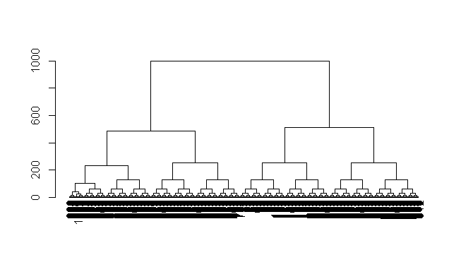
dend1000

dendextend: a package for visualizing, adjusting, and comparing dendrograms (based on a paper from “bioinformatics”)

This post on the dendextend package is based on my recent paper from the journal bioinformatics (a link to a stable DOI). The paper was published just last week, and since it is released as CC-BY, I am permitted (and delighted) to republish it here in full:

abstract

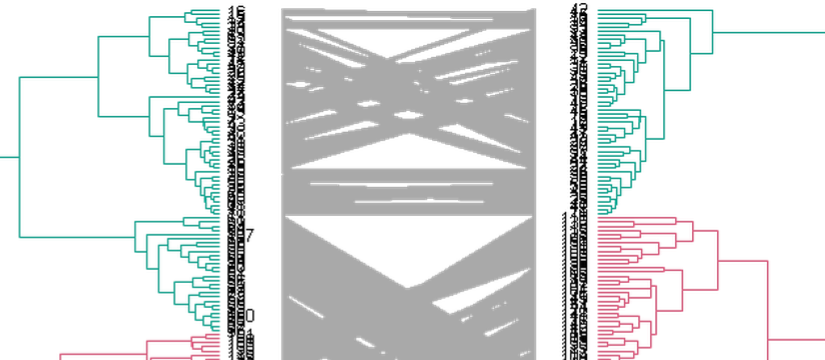
Summary: dendextend is an R package for creating and comparing visually appealing tree diagrams. dendextend provides utility functions for manipulating dendrogram objects (their color, shape, and content) as well as several advanced methods for comparing trees to one another (both statistically and visually). As such, dendextend offers a flexible framework for enhancing R’s rich ecosystem of packages for performing hierarchical clustering of items.

Availability: The dendextend R package (including detailed introductory vignettes) is available under the GPL-2 Open Source license and is freely available to download from CRAN at: (https://cran.r-project.org/package=dendextend)

Contact: [email protected]

Continue reading “dendextend: a package for visualizing, adjusting, and comparing dendrograms (based on a paper from “bioinformatics”)”

dendextend version 1.0.1 + useR!2015 presentation

When using the dendextend package in your work, please cite it using:

Tal Galili (2015). dendextend: an R package for visualizing, adjusting, and comparing trees of hierarchical clustering. Bioinformatics. doi:10.1093/bioinformatics/btv428

My R package dendextend (version 1.0.1) is now on CRAN!

The dendextend package Offers a set of functions for extending dendrogram objects in R, letting you visualize and compare trees of hierarchical clusterings. With it you can (1) Adjust a tree’s graphical parameters – the color, size, type, etc of its branches, nodes and labels. (2) Visually and statistically compare different dendrograms to one another.

The previous release of dendextend (0.18.3) was half a year ago, and this version includes many new features and functions.

To help you discover how dendextend can solve your dendrogram/hierarchical-clustering issues, you may consult one of the following vignettes:

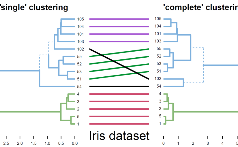
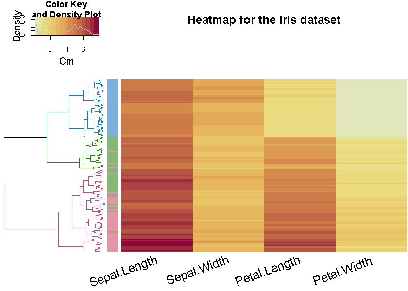
Here is an example figure from the first vignette (analyzing the Iris dataset)

iris_heatmap_dend


This week, at useR!2015, I will give a talk on the package. This will offer a quick example, and a step-by-step example of some of the most basic/useful functions of the package. Here are the slides:


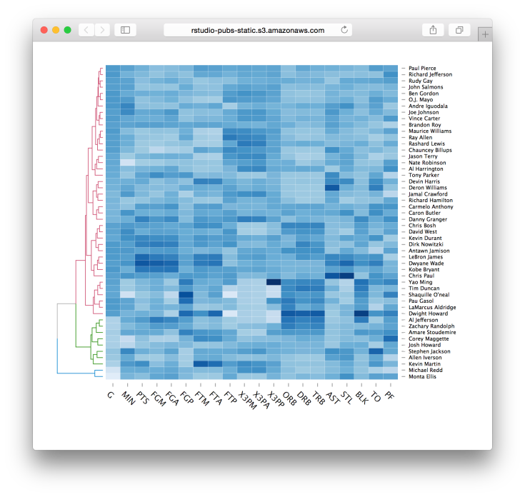
Lastly, I would like to mention the new d3heatmap package for interactive heat maps. This package is by Joe Cheng from Rstudio, and integrates well with dendrograms in general and dendextend in particular (thanks to some lovely github-commit-discussion between Joe and I). You are invited to see lively examples of the package in the post at the RStudio blog. Here is just one quick example:

d3heatmap(nba_players, colors = “Blues”, scale = “col”, dendrogram = “row”, k_row = 3)

d3heatmap

Setting Rstudio server using Amazon Web Services (AWS) – a step by step (screenshots) tutorial

(this is a guest post by Liad Shekel)

Amazon Web Services (AWS) include many different computational tools, ranging from storage systems and virtual servers to databases and analytical tools. For us R-programmers, being familiar and experienced with these tools can be extremely beneficial in terms of efficiency, style, money-saving and more.

In this post we present a step-by-step screenshot tutorial that will get you to know Amazon EC2 service. We will set up an EC2 instance (Amazon virtual server), install an Rstudio server on it and use our beloved Rstudio via browser (all for free!). The slides below will also include an introduction to linux commands (basic), instructions for connecting to a remote server via ssh and more. No previous knowledge is required.

Useful links:

  1. Set up an AWS account (do not worry about the credit card details, you will not be charged for any of  our actions) – the steps are presented in the slides below.
  2. Windows users: download MobaXterm (or any other ssh client software).
    Mac users: make sure you are familiar with the terminal (cause I’m not).


A step by step (screenshots) tutorial for upgrading R on Windows

tl;dr

If you are running R on Windows you can easily upgrade to the latest version of R using the installr package. Simply run the following code:

# installing/loading the latest installr package:
install.packages("installr"); library(installr) # install+load installr

updateR() # updating R.

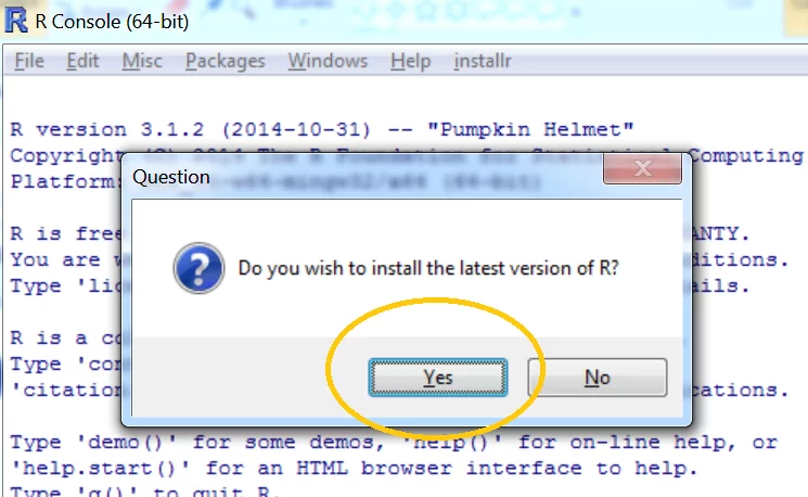
Running “updateR()” will detect if there is a new R version available, and if so it will download+install it (etc.). just press “next”, “OK”, and “Yes” on everything…

A GUI interface to updating R on Windows

Starting from installr version 0.15.0, the upgradingprocess can be done with a click-on-menus GUI interface. Here is how to use it.

Continue reading “A step by step (screenshots) tutorial for upgrading R on Windows”

The ensurer package (validation inside pipes)

Guest post by Stefan Holst Milton Bache on the ensurer package.

If you use R in a production environment, you have most likely experienced that some circumstances change in ways that will make your R scripts run into trouble. Many things can go wrong; package updates, external data sources, daylight savings time, etc. There is a general increasing focus on this within the R community and words like “reproducibility”, “portability” and “unit testing” are buzzing big time. Many really neat solutions are already helping a lot: RStudio’s Packrat project, Revolution Analytic’s “snapshot” feaure, and Hadley Wickham’s testthat package to name a few. Another interesting package under development is Edwin de Jonge’s “validate” package.

I found myself running into quite a few annoying “runtime” moments, where some typically external factors break R software, and more often than not I spent just too much time tracking down where the bug originated. It made me think about how best to ensure that vulnarable statements behaves as expected and how to know exactly where and when things go wrong. My coding style is heaviliy influenced by the magrittr package’s pipe operator, and I am very happy with the workflow it generates:

data <-
  read_external(...) %>%
  make_transformation(...) %>%
  munge_a_little(...) %>%
  summarize_somehow(...) %>%
  filter_relevant_records(...) %T>%
  maybe_even_store

It’s like a recipe. But the problem is that I found no existing way of tagging potentially vulnarable steps in the above process, leaving the choice of doing nothing, or breaking it up. So I decided to make “ensurer”, so I could do:

data <-
  read_external(...) %>%
  ensure_that(all(is.good(.)) %>%
  make_transformation(...) %>%
  ensure_that(all(is.still.good(.))) %>%
  munge_a_little(...) %>%
  summarize_somehow(...) %>%
  filter_relevant_records(...) %T>%
  maybe_even_store

Now, I don’t have a blog, but Tal Galili has been so kind to accept the ensurer vignette as a post for r-bloggers.com. I hope that ensurer can help you write better and safer code; I know it has helped me. It has some pretty neat features, so read on and see if you agree!

Continue reading “The ensurer package (validation inside pipes)”