New edition of "R Companion to Applied Regression" – by John Fox and Sandy Weisberg

Just two hours ago, Professor John Fox has announced on the R-help mailing list of a new (second) edition to his book “An R and S Plus Companion to Applied Regression”, now title . “An R Companion to Applied Regression, Second Edition”.

John Fox is (very) well known in the R community for many contributions to R, including the car package (which any one who is interested in performing SS type II and III repeated measures anova in R, is sure to come by), the Rcmdr pacakge (one of the two major GUI’s for R, the second one is Deducer), sem (for Structural Equation Models) and more.  These might explain why I think having him release a new edition for his book to be big news for the R community of users.

In this new edition, Professor Fox has teamed with Professor Sandy Weisberg, to refresh the original edition so to cover the development gained in the (nearly) 10 years since the first edition was written.

Here is what John Fox had to say:

Dear all,

Sandy Weisberg and I would like to announce the publication of the second
edition of An R Companion to Applied Regression (Sage, 2011).

As is immediately clear, the book now has two authors and S-PLUS is gone
from the title (and the book). The R Companion has also been thoroughly
rewritten, covering developments in the nearly 10 years since the first
edition was written and expanding coverage of topics such as R graphics and
R programming. As before, however, the R Companion provides a general
introduction to R in the context of applied regression analysis, broadly
construed. It is available from the publisher at (US) or (UK), and from Amazon (see here)

The book is augmented by a web site with data sets, appendices on a variety of topics, and more, and it associated with the car package on CRAN, which has recently undergone an overhaul.

Regards,
John and Sandy

Continue reading “New edition of "R Companion to Applied Regression" – by John Fox and Sandy Weisberg”

Visualization of regression coefficients (in R)

Update (07.07.10): The function in this post has a more mature version in the “arm” package. See at the end of this post for more details.
* * * *

Imagine you want to give a presentation or report of your latest findings running some sort of regression analysis. How would you do it?

This was exactly the question Wincent Rong-gui HUANG has recently asked on the R mailing list.

One person, Bernd Weiss, responded by linking to the chapter “Plotting Regression Coefficients” on an interesting online book (I have never heard of before) called “Using Graphs Instead of Tables” (I should add this link to the free statistics e-books list…)

Letter in the conversation, Achim Zeileis, has surprised us (well, me) saying the following

I’ve thought about adding a plot() method for the coeftest() function in the “lmtest” package. Essentially, it relies on a coef() and a vcov() method being available – and that a central limit theorem holds. For releasing it as a general function in the package the code is still too raw, but maybe it’s useful for someone on the list. Hence, I’ve included it below.

(I allowed myself to add some bolds in the text)

So for the convenience of all of us, I uploaded Achim’s code in a file for easy access. Here is an example of how to use it:

source("https://www.r-statistics.com/wp-content/uploads/2010/07/coefplot.r.txt")

data("Mroz", package = "car")
fm <- glm(lfp ~ ., data = Mroz, family = binomial)
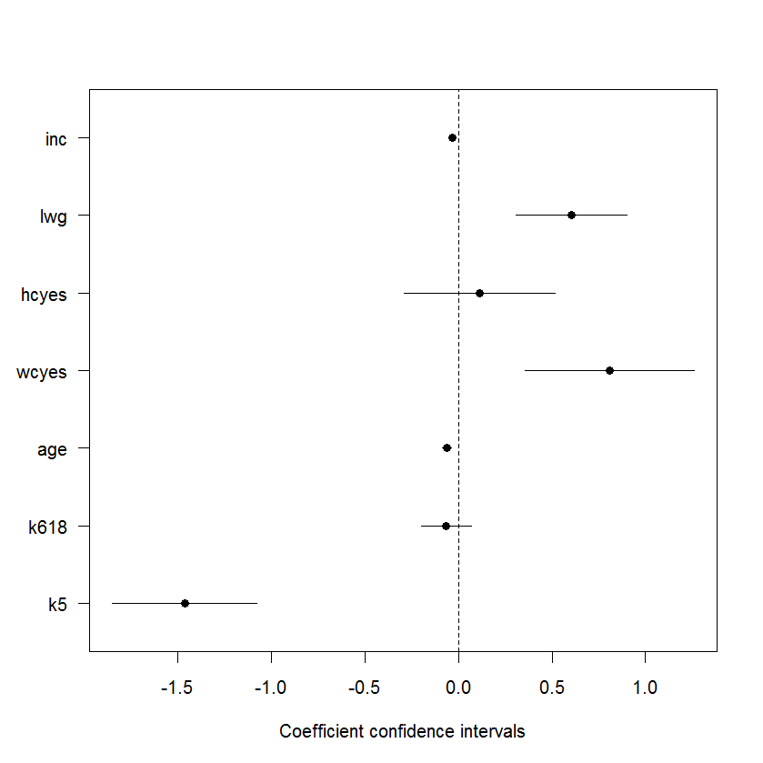
coefplot(fm, parm = -1)

Here is the resulting graph:

I hope Achim will get around to improve the function so he might think it worthy of joining his"lmtest" package. I am glad he shared his code for the rest of us to have something to work with in the meantime 🙂

* * *

Update (07.07.10):
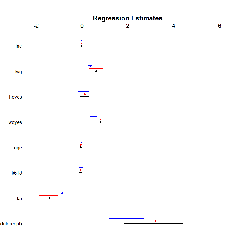
Thanks to a comment by David Atkins, I found out there is a more mature version of this function (called coefplot) inside the {arm} package. This version offers many features, one of which is the ability to easily stack several confidence intervals one on top of the other.

It works for baysglm, glm, lm, polr objects and a default method is available which takes pre-computed coefficients and associated standard errors from any suitable model.

Example:
(Notice that the Poisson model in comparison with the binomial models does not make much sense, but is enough to illustrate the use of the function)

library("arm")
data("Mroz", package = "car")
M1<-      glm(lfp ~ ., data = Mroz, family = binomial)
M2<- bayesglm(lfp ~ ., data = Mroz, family = binomial)
M3<-      glm(lfp ~ ., data = Mroz, family = binomial(probit))
coefplot(M2, xlim=c(-2, 6),            intercept=TRUE)
coefplot(M1, add=TRUE, col.pts="red",  intercept=TRUE)
coefplot(M3, add=TRUE, col.pts="blue", intercept=TRUE, offset=0.2)

(hat tip goes to Allan Engelhardt for help improving the code, and for Achim Zeileis in extending and improving the narration for the example)

Resulting plot

* * *
Lastly, another method worth mentioning is the Nomogram, implemented by Frank Harrell'a rms package.